Transformers
Transformers have generated headlines both figuratively and literally. They can produce text (or chat with you) more or less on any topic and the result looks astonishingly authentic (i.e. as if produced by a human). There are, of course, hillarious examples where the machine overachieves on its smarts. Below is an example from a test session of GPT-3 for generating chat bot responses on a medical service’s website:

Since Open AI released GPT-3 as a SaaS service, I have heard about hundreds of startups trying to monetize the technology. The catch is, of course, how can you trust the technology to do what you want. With very limited understanding of the model’s operating logic, it is rather difficult to use it without human supervision. In our (AlphaChat) experience, you can use GPT-3 as a tool for generating text or phrases and then have humans to validate that the result is what was expected. In that sense GPT-3 is not a magic wand, but rather a bottomless mixed bag of authentic and fool’s gold.
For a deeper excursion into the interpretability of transformers I suggest to check these excellent papers:
A Mathematical Framework for Transformer Circuits
In-context Learning and Induction Heads
High level architecture
In order to demystify machine learning models, it is best to look under the hood. When doing this I often feel like Alice in wonderland exclaiming “You’re nothing but a pack of cards!”. That is because despite all their great achievements and our anthropomorphic expectations about the complicated reasoning capabilities of advanced deep learning systems, you will eventually discover that “You’re nothing but a bunch of matrix multiplications!”. Still, facing the undeniable effectiveness of deep learning in solving extremely complicated problems such as protein folding, we have to stay humble. We should remind ourselves that the implementational mechanism (matrix multiplications) is not a description of the algorithm that the transformer is executing. Similarly, knowing that neurons use synapses to exchange information in the brain does not tell us what operations the brain is performing with this information.
Recent efforts to obtain a higher-level description of the operations that the transformer is implementing have been somewhat successful. For example, it seems that the attention heads copy information about previous tokens (the source) to the tokens that follow them (the destination) so that the embedding vector of the destination tokens will contain information about bigrams (a pair of adjacent tokens):
In our previous paper, we discovered a special kind of attention head – which we named induction heads – in two layer attention-only models. Induction heads are implemented by a circuit consisting of a pair of attention heads in different layers that work together to copy or complete patterns. The first attention head copies information from the previous token into each token. This makes it possible for the second attention head to attend to tokens based on what happened before them, rather than their own content. Specifically, the second head (which we call the “induction head”) search for a previous place in the sequence where the present token
Aoccurred and attends to the next token (call itB), copying it and causing the model to be more likely to outputBas the next token. That is, the two heads working together cause the sequence…[A][B]…[A]to be more likely to be completed with[B].https://transformer-circuits.pub/2022/in-context-learning-and-induction-heads/index.html
We have to conclude that while understanding how the network is constructed and how it operates on the lower level (i.e. on the level of artifical neural units and weights) we are mostly left in the dark about the higher-level algorithmic description of the solution that it is implementing. In a way, we are creating an artifical brain that can solve problems, but is doing it in a very messy way that is quite incomprehensible to us. To me, it resembles the messiness of the mode of operation in a living cell and in a biological brain.
Residual stream
A proposed here, I find it very useful to approach the architecture of the transformer from the viewpoint of the residual stream as its backbone. Residual stream is the river of information that carries data about the statistical relantionships between tokens. All layers of the transformer get their input from this stream and write their output back to the stream. You can think about it as a sketchpad where different layers of the network (GPT-3 has e.g. 96 attention layers) can make adjustments, add and delete information with the sole objective of being able to predict the next token based on the context of previous tokens.
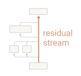
One of the main features of the high level architecture of a transformer is that each layer adds its results into what we call the “residual stream.” The residual stream is simply the sum of the output of all the previous layers and the original embedding. We generally think of the residual stream as a communication channel, since it doesn’t do any processing itself and all layers communicate through it.
https://transformer-circuits.pub/2021/framework/index.html
Information in the final layer of the residual stream is used to calculate the probability of each known token being the next one in the sequence. In essence, the transformer is a model that predicts the probability of the next token’s identity depending on the sequence of tokens that have preceded it. In order to do this effectively in the context of natural language, the model needs to be able to approximate grammatical and semantic relations between words as otherwise it would not be able to generate fluent and human-readable text.
To me, the most important revelation from the papers referenced above was that a key job of the attention heads is to modify the embedding of each token so that it will contain information about it’s associations with preceding tokens. Thus, when looking up a single token via the query-key mechanism (detailed below), the attention head can retrieve an embedding which already contains information about the token that will follow it.
[induction heads] search the context for previous instances of the present token, attend to the token which would come next if the pattern repeated, and increase its probability. Induction heads attend to tokens that would be predicted by basic induction (over the context, rather than over the training data).
https://transformer-circuits.pub/2022/in-context-learning-and-induction-heads/index.html
The biggest contribution of the transformer architecture is the multi-headed attention mechanism. That is why I took some time to expand the associated entities in terms of their properties and intuitive meaning below. In order to make sure I understood multiheaded attention in sufficient detail, I took the trouble of expressing relevant operations in R code so as to arrive at matrix multiplications that would produce the output with correct dimensions.
Attention mechanism
A residual block is composed of an attention component with multiple attention heads (GPT-3 has 96 attention heads per attention layer) and an MLP component. Residuals blocks are arranged sequentially as layers in a typical deep neural net.
https://transformer-circuits.pub/2021/framework/index.html
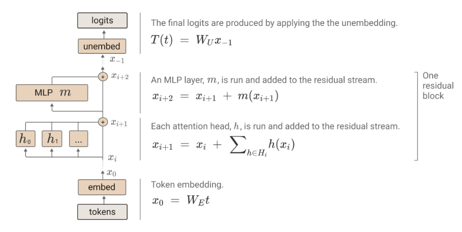
Below is an annotation of the variables in the figure above.
$t$ is a matrix with dimensions [n_context, n_vocab] i.e. one row per each position in the text and columns corresponding to known tokens in one-hot encoding.
$W_E$ is a learnable matrix with dimensions [d_model, n_vocab] where each column represents the embedding vector of the corresponding token. $W_E$ transforms one-hot encoded tokens into corresponding embeddings.
$x_i$ with dimensions [d_model, n_context] is the hidden state of the model after the i-th residual component.
$W_U$ [n_vocab, d_model] is the unembedding matrix that is used to produce logits.
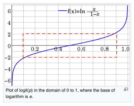
The logit (logarithm of odds) is defined as $ln(\frac{p}{1-p})$ where $p$ is a probability in the range $[0,1]$. Logits are positive when p > 0.5 and negative when p < 0.5. Note that $logit(p)$ is a virtually linear function of $p$ in the range $0.1 < p < 0.9$ (represented by the red rectangle).
https://en.wikipedia.org/wiki/Logit
Below is a demonstration (in R code) how to get token embeddings from one-hot encoded tokens.
# W_E token embeddings [d_model, n_vocab]
# one token per column
d_model = 3
n_vocab = 2
W_E <- matrix(c(c(1:d_model), c(1:d_model)*10), c(d_model, n_vocab))

# output:
     [,1] [,2]
[1,]    1   10
[2,]    2   20
[3,]    3   30

# one-hot encodings for tokens "a" and "b" when n_vocab=2
a <- c(1,0)
b <- c(0,1)

# t [n_vocab, n_context]
# columns correspond to positions in (con)text and rows to onehot encoded tokens
# given a vocabulary of tokens "a" and "b", the current instantiation of context t
# refers to the following sequence of tokens: "a b b a" i.e. d_context=4
d_context = 4
t <- matrix(c(a, b, b, a), c(n_vocab, d_context))

# decorated output:
     [,1] [,2] [,3] [,4]
[1,]    1    0    0    1
[2,]    0    1    1    0
       "a"  "b"  "b"  "a"

# x_0 [n_model, n_context] is a sequence of token embeddings where each column corresponds to a position in the sequence and the rows correspond to the embedding/model space
# i.e. W_E [d_model, n_vocab] %*% t [n_vocab, n_context] = x_0 [d_model, n_context]
x_0 <- W_E %*% t

# output:
     [,1] [,2] [,3] [,4]
[1,]    1   10   10    1
[2,]    2   20   20    2
[3,]    3   30   30    3

# A %*% B (in R) or AB (in traditional notation) represent standard matrix multiplication.
# For each row of A calculate the dot products with each column of B.
# Thus, the dimensions of the resulting matrix AB are [A.nrow(), B.ncol()]
#
# pseudocode:
# result = matrix(A.nrow(), B.ncol())
# for a_row in range(A.nrow()):
#   for b_col in range(B.ncol()):
#     result[a_row, b_col] = sum(A[a_row,:] * B[:,b_col])

# decorated example of the matrix multiplication process:

            W_E  %*%  t
      [,1] [,2]             [,1] [,2] [,3] [,4]
[1,]    1   10        [1,]    1    0    0    1    =
[2,]    2   20        [2,]    0    1    1    0
[3,]    3   30

sum(W_E[1,]*t[,1])=1   sum(W_E[1,]*t[,2])=10   sum(W_E[1,]*t[,3])=10  sum(W_E[1,]*t[,4])=1
sum(W_E[2,]*t[,1])=2   sum(W_E[2,]*t[,2])=20   sum(W_E[2,]*t[,3])=20  sum(W_E[2,]*t[,4])=2
sum(W_E[3,]*t[,1])=3   sum(W_E[2,]*t[,2])=30   sum(W_E[2,]*t[,3])=30  sum(W_E[2,]*t[,4])=3
Below is a figure summarizing the attention mechanism. It uses a slightly different notation for learnable weight matrices where Ql = WQh, Kl = WKh and Vl = WVh.
https://thegradient.pub/transformers-are-graph-neural-networks/
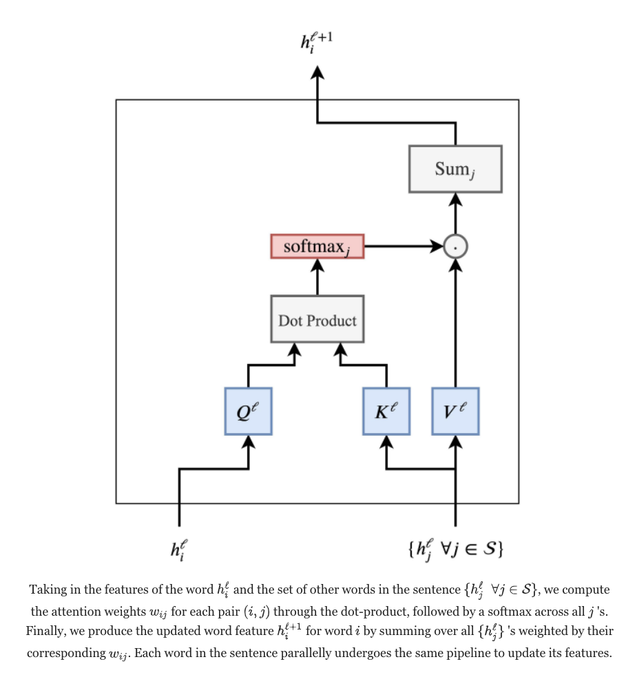
WQh, WKh, WVh are matrices with dimensions [d_head, d_model] corresponding to query, key, and value weights of attention head $h$.
$h^{l}_{i}$ is a vector of activations for token i in layer $l$.
The query vector is produced by projecting \(h^{l}_{i}\) from model space d_model to attention head space d_head (128 in GPT-3) via the learnable $W_{Q}^{h^{l}}$ matrix. In other words, $W_{Q}^{h^{l}}$ is a matrix of weights for projecting the current token from model space to attention space in layer $l$ for attention head $h$.
The key vector key with dimensions [d_head, 1] for token $j$ is obtained analogously by multiplying the $W_{K}^{h^{l}}$ matrix with token activations $h^{l}_{j}$ .
https://thegradient.pub/transformers-are-graph-neural-networks/
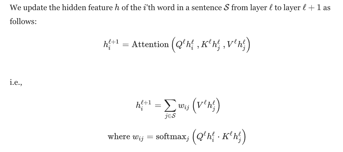
The softmax-normalized vector of dot-products (referred to as qk_softmaxed in the code below) between the single query $i$ and every key $j$ represents attention scores in the range $[0, 1]$ and adding up to a total of 1. This vector determines how much the features of each token $j$ affect the features of token $i$. This is the “focus” or “attention” that is spent on other tokens $j$ when calculating the activation of token $i$ that will enter hidden layer $l+1$. It constitutes the lookup mechanism of the transformer that can look for tokens that are in some respect similar to the query token in the given context. This context-dependent lookup mechanism is also the basis for the priming of transformers whereby you can feed the transformer with some text that acts as an instruction to direct its output. In AlphaChat, for example, we have used priming such as “make a list of questions that you can ask about car insurance policy from a customer service representative working in an insurance company” to autogenerate training phrases for the bot (of course we had someone validate the output before it was added to the training data). Since attention heads can incorporate information about associated tokens into a single embedding vector using different dimensions of the vector as separate memory locations, the query-key lookup mechanism can focus on different regions of the embedding vector to look up different information about the token in question.
Below is a demonstration (in R code) how to compute the output of the attention layer.
# no. of preceding tokens that are used as context to predict the next token
d_context <- 7
# model space (aka token embedding space) dimensions extend from several hundred in small models to tens of thousands in larger models
d_model <- 5
# attention head space typically extends to 64 to 128 dimensions
d_head <- 3

# hidden state at layer l [d_model, d_context]
h <- matrix(rnorm(d_model*d_context, 0, 1), c(d_model, d_context))

# select one position from context as the query
i <- 6
# a [d_model, 1] matrix (a column vector) of activations for token i
h_i <- matrix(h[,i], c(d_model, 1))
# generate a [d_head, d_model] matrix of randomly chosen values with mean 0 and sd 0.5
W_Q <- matrix(rnorm(d_head*d_model,0,0.5), c(d_head, d_model))
# a column vector [d_head, 1] of query activations for attention head
query <- W_Q %*% h_i

# initialize the query-key dot product vector to zeros
qk <- rep(0, d_context)

# W_K is the key weight matrix for attention head h
W_K <- matrix(rnorm(d_head*d_model,0,0.5), c(d_head, d_model))
for(j in 1:d_context){
  # calculate the query-key product for token i with
  # each token/position j in context
  h_j <- h[,j]
  key <- W_K %*% h_j

  # the dot product between query i and key j
  qk[j] <- sum(query * key)

  # Note that there is no a-priori reason for the maximum of qk
  # to be located at qk[i] (i.e. when j==i) unless the projection
  # matrices W_Q and W_K are correlated. Multiplication of the same
  # input vector with different matrices will yield query and key
  # vectors with arbitrarily divergent values.
}

# normalize {a} into a range between 0 and 1
softmax <- function(a){
  exponents <- exp(a)
  exponents / sum(exponents)
}

qk_softmaxed <- softmax(qk)

# initialize the attention signal for token i to zeros
attention_signal_for_token_i <- rep(0, d_head)

# W_V is the value weight matrix for attention head h
W_V <- matrix(rnorm(d_head*d_model,0,0.5), c(d_head, d_model))

# loop through all tokens in context
for(j in 1:d_context){
  h_j <- h[,j]
  value <- W_V %*% h_j
  # the impact of the {value} of token {j} on the activation of token {i}
  # (i.e. on {attention_signal_for_token_i}) is proportional to qk_softmaxed[j]
  attention_signal_for_token_i <- attention_signal_for_token_i + qk_softmaxed[j] * value
}

# learnable weights to project attention signal from head space to model space
W_OV <- matrix(rnorm(d_head*d_model,0,0.5), c(d_model, d_head))

# output of the current layer into the residual stream.
# a [d_model, 1] matrix (a column vector) of activation signals
# to be added to the embedding of the {i}-th token in the residual
# stream's {i}-th column.
output <- W_OV %*% attention_signal_for_token_i

# note! in the real-life implementation, the outputs of attention heads are concatenated and W_OV are concatenated and multiplied with
In a single layer, multiple attention heads operate independently (i.e. they get identical input from the residual stream) and in parallel (each adds its output to the token embeddings in the residual stream).
The residual stream is a high-dimensional vector space. In small models, it may be hundreds of dimensions; in large models it can go into the tens of thousands. This means that layers can send different information to different layers by storing it in different subspaces. This is especially important in the case of attention heads, since every individual head operates on comparatively small subspaces (often 64 or 128 dimensions), and can very easily write to completely disjoint subspaces and not interact.
Once added, information persists in a subspace unless another layer actively deletes it. From this perspective, dimensions of the residual stream become something like “memory” or “bandwidth”. The original token embeddings, as well as the unembeddings, mostly interact with a relatively small fraction of the dimensions. 6 This leaves most dimensions “free” for other layers to store information in.
https://transformer-circuits.pub/2021/framework/index.html
MLP layers
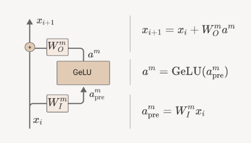
Understanding the function of MLP layers has been more difficult although they make up two thirds of a standard transformer’s parameters. MLP-s are single layer networks which project token embeddings retrieved from the residual stream to a higher dimensional space, apply the activation function and project the resulting activations back to the embedding space and, finally, add the result back to the residual stream.
There seems to be evidence that MLP layers perform memory management functions:
we’ve seen hints that some MLP neurons and attention heads may perform a kind of “memory management” role, clearing residual stream dimensions set by other layers by reading in information and writing out the negative version
https://transformer-circuits.pub/2021/framework/index.html
There are also suggestions that the MLP layers might enable the network to model a wider array of functions (i.e. behave as a universal approximator).
Implementational details
Numerical stability
Layer normalization is used after each attention and MLP layer to re-scale token activation values in the residual stream into a stable distribution (centered around zero and with standard deviation close to 1), making transformers easier to train. Specifically, layer normalization recenters all activation values $a_i$ in layer $l$ to the mean activation (of layer $l$) and rescales them by the standard deviation (of activations in layer $l$). In addition, layer norm learns an adaptive gain factor $g_i$ and a bias $b_i$ for each unit $i$ in layer $l$.
$h_i = \frac{g_i}{\sigma^l}(a_i-\mu^l)+b_i$
This is important, because individual attention heads can produce signals with different magnitudes, which can lead to highly variable activation values when the outputs of multiple attention layers are added to the residual stream. The scale and distribution of hidden unit activation values has a significant impact on the propagation of the error gradient and it is generally believed that various forms of normalization ease the back-propagation of the gradients. Gradients that are too large (aka “exploding” gradients) tell the gradient descent algorithm to update the weights by a lot at a time, which will change the model’s output too much and prevent consistent navigation of the error landscape. Too small weights will diminish gradients (known as the vanishing gradient problem) and result in tiny updates to the weights. Vanishing gradients cause the training process to gets stuck in a local minimum or become very slow to progress. See here for a treatment of the gradient instability topics by Andrew Ng (btw - I got the basics of machine learning from his Coursera course).
You can think about this literally in terms of hill climbing. Let’s assume that you are an incredibly advanced (and, of course, intelligent) life form that tries to minimize oxygen in its surroundings. You prefer the thin air of high altitudes and move around with a fancy teleportation device. So your goal is to climb the highest hilltop and you can move towards it one jump at a time. If your jumps are too large, you will teleport yourself over the hill without being able to reach the top. On the other hand, if your jumps are too small, it will take forever to reach the hilltop. In the neural net world, controlling the distribution of network parameter values (i.e. the size and variability of learnable weights) and adjusting the learning rate (the key parameter in the gradient descent algorithm), are the keys to ensuring correct step size for updating the models parameters.
Parallelization
In the code example above I was using a for loop to calculate the dot product between token $i$ with all tokens $j$. I find this presentation algorithmically descriptive, but the implementation would be painfully slow to run on a computer aided with GPU cards. In real life implementations, the for loops are replaced by matrix multiplications where the weights of all attention heads in a single layer are concatenated into a single matrix. Multiplying, for example, such WKl matrix of layer $l$ with the token embedding matrix at layer $l$ will give you a matrix containing the keys for all tokens $j$ for all heads $h$ in layer $l$. In essence then, these large matrix multiplications are an optimization to GPU-architecture, which is very important if you want to save time and money when training these huge networks.
Positional encoding
Positional information about token’s location in the context sequence is provided by positional encoding vectors that are different for each position and get added to the token embeddings.
At their most basic level, positional embeddings are kind of like token addresses. Attention heads can use them to prefer to attend to tokens at certain relative positions, but they can also do much more.
https://transformer-circuits.pub/2021/framework/index.html
It seems that attention heads sometimes copy positional embeddings from attented tokens to the current token and also transpose them (e.g. move forward) in order to facilitate prediction of the next token.
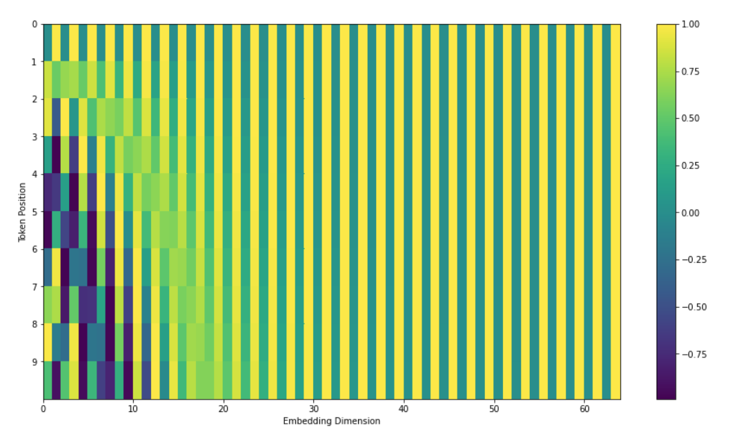
A nice illustration of positional encoding is provided below (a link to the code):
https://jalammar.github.io/illustrated-transformer/